Analyze a post-training Bernoulli-Bernoulli RBM

This script shows how to analyze the RBM after having trained it.

import matplotlib.pyplot as plt
import torch

device = torch.device("cpu")
dtype = torch.float32

Load the dataset

We suppose the RBM was trained on the dummy.h5 dataset file, with 60% of the train dataset. By default, the dataset splitting is seeded. So just putting the same train_size and test_size ensures having the same split for analysis. This behaviour can be changed by setting a different value to the seed keyword.

from rbms.dataset import load_dataset

train_dataset, test_dataset = load_dataset(
    "dummy.h5", train_size=0.6, test_size=0.4, device=device, dtype=dtype
)
num_visibles = train_dataset.get_num_visibles()

U_data, S_data, V_dataT = torch.linalg.svd(
    train_dataset.data - train_dataset.data.mean(0)
)
proj_data = train_dataset.data @ V_dataT.mT / num_visibles**0.5
proj_data = proj_data.cpu().numpy()

Load the model.

First, we want to know which machines have been saved

from rbms.utils import get_saved_updates

filename = "RBM.h5"
saved_updates = get_saved_updates(filename=filename)
print(f"Saved updates: {saved_updates}")

Saved updates: [    1     2     3     4     5     7     8    10    13    16    20    25
    31    39    49    61    75    94   116   145   180   223   277   344
   427   531   659   765   819   849   990  1017  1024  1262  1567  1568
  1946  2118  2391  2416  2655  3000  3725  3799  4625  5743  7033  7131
  8853 10992 13648 16946 18038 21040 26123 31967 32434 40270 42529 50000]

Now we will load the last saved model as well as the permanent chains during training Only the configurations associated to the last saved model have been saved for the permanent chains. We also get access to the hyperparameters of the RBM training as well as the time elapsed during the training.

from rbms.io import load_model

params, permanent_chains, training_time, hyperparameters = load_model(
    filename=filename, index=saved_updates[-1], device=device, dtype=dtype
)

print(f"Training time: {training_time}")
for k in hyperparameters.keys():
    print(f"{k} : {hyperparameters[k]}")

Training time: 4915.106016874313
batch_size : 2000
gibbs_steps : 5
learning_rate : 0.01

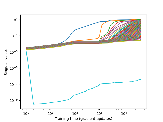
To follow the training of the RBM, let’s look at the singular values of the weight matrix

from rbms.utils import get_eigenvalues_history

grad_updates, sing_val = get_eigenvalues_history(filename=filename)

fig, ax = plt.subplots(1, 1)
ax.plot(grad_updates, sing_val)
ax.set_xlabel("Training time (gradient updates)")
ax.set_ylabel("Singular values")
ax.loglog()
fig.show()

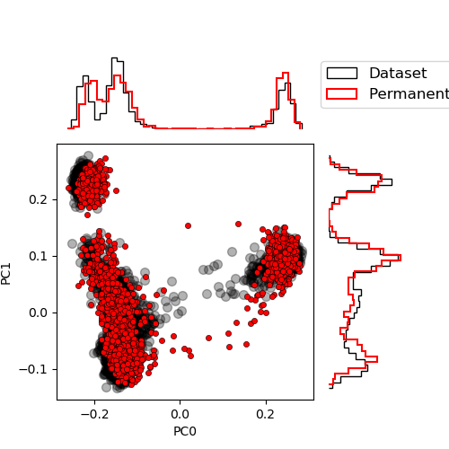
Let’s compare the permanent chains to the dataset distribution. To do so, we project the chains on the first principal components of the dataset.

from rbms.plot import plot_PCA

proj_pc = permanent_chains["visible"] @ V_dataT.mT / num_visibles**0.5

plot_PCA(
    proj_data,
    proj_pc.cpu().numpy(),
    labels=["Dataset", "Permanent chains"],
)

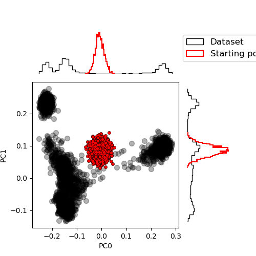
Sample the RBM

Another interesting thing is to compare generated samples starting from random configurations

from rbms.sampling.gibbs import sample_state

num_samples = 2000
chains = params.init_chains(num_samples=num_samples)
proj_gen_init = chains["visible"] @ V_dataT.mT / num_visibles**0.5
plot_PCA(
    proj_data,
    proj_gen_init.cpu().numpy(),
    labels=["Dataset", "Starting position"],
)
plt.tight_layout()

/home/nbereux/work/rbms/examples/plot_generated_samples.py:100: UserWarning: Tight layout not applied. tight_layout cannot make Axes width small enough to accommodate all Axes decorations
  plt.tight_layout()

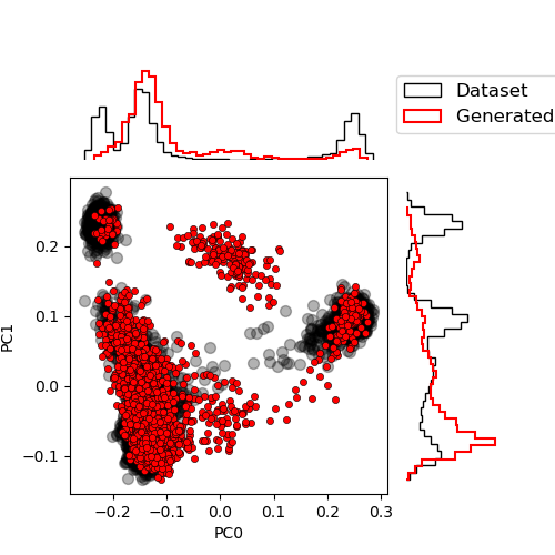
We can now sample those chains and compare again the distribution

n_steps = 100
chains = sample_state(gibbs_steps=n_steps, chains=chains, params=params)

proj_gen = chains["visible"] @ V_dataT.mT / num_visibles**0.5
plot_PCA(
    proj_data,
    proj_gen.cpu().numpy(),
    labels=["Dataset", "Generated samples"],
)

Compute the AIS estimation of the log-likelihood.

For now, we only looked at a qualitative evaluation of the model

from rbms.partition_function.ais import compute_partition_function_ais
from rbms.utils import compute_log_likelihood

log_z_ais = compute_partition_function_ais(num_chains=2000, num_beta=100, params=params)

print(
    compute_log_likelihood(
        train_dataset.data, train_dataset.weights, params=params, log_z=log_z_ais
    )
)

-387.64599609375